Charge Flipping in
GSAS-II - sucrose
Prerequisite:
In this exercise you will use GSAS-II to solve the structure of sucrose from powder diffraction data via charge flipping. This structure was originally solved from single crystal data in the space group P21. It is a difficult exercise to complete as the charge flipping does not always yield a solution and to even have a chance the Pawley refinement must be done with particular care. We have given a route that sometimes works.
If you have not done so already, start GSAS-II and open the GSAS-II project file (I called it sucrose.gpx) you saved from the third part of the peak fitting-indexing exercise. If you didn’t do that exercise, do it now.
Step 1: Setup for Pawley refinement
There are a number of steps that must be done in preparation for a Pawley refinement after having completed the unit cell indexing and new phase creation. These cover two things: one is to prepare the powder pattern (reset limits, etc.) and the other is to prepare the phase for the refinement.
1. Select Limits in the GSAS-II data tree for the PWDR data set and expand the plot so that the region near d=1.0Å is readily seen. This is ~24deg 2Q. There is an area relatively clear of peaks that makes a good place to end the calculations with a reflection set of dmin ~1Å resolution needed for charge flipping. Enter 23.55 for Tmax as the upper limit and make a note of the exact d-spacing (1.0125Å) using the mouse cursor on the plot.
2. Select Instrument Parameters and uncheck all Refine flags and do Operations/Reset profile to recover the default values. The peak fitting done earlier is over a much more limited range of 2Q giving values that might not extrapolate well over the wider range to be used in the Pawley refinement. We will refine them again later.
3. Select Sample Parameters and uncheck refinement of Histogram scale factor. While you are here set Goniometer radius to 1000.
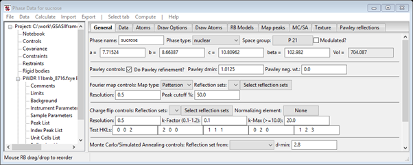
4. Go to Phases/sucrose to find the Pawley controls. Check the Do Pawley refinement box and enter the d-spacing (1.0125) into the Pawley dmin box. Set the Pawley neg. wt. to 0.001
When done the General tab should look like
Next find the Data tab; it will be empty except for some text. Do Edit Phase/Add powder histograms; a dialog box will appear
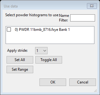
Select the only choice and press OK; the desired data set will be added to this phase for analysis. The data tab now shows the new data set.
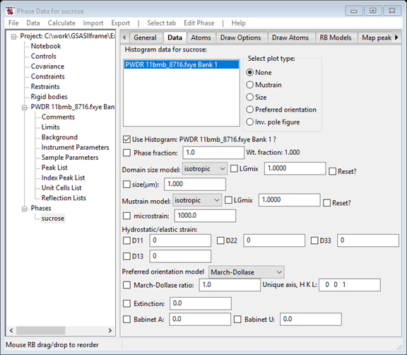
I’ve stretched the window slightly to see the entire contents. This is the location for all the phase dependent parameters for this histogram. Notice that it includes phase fraction, size & mustrain as well as preferred orientation, elastic strain and extinction corrections. The Babinet correction is intended for protein work where a significant region of the structure is disordered solvent. There are buttons for plotting size and mustrain surfaces as well as preferred orientation correction curves.
Next find the Pawley reflections tab; it will be empty except for column headings. Do Operations/Pawley create; this makes the reflection set over the range covered by setting Pawley dmin. The table should list reflections 0~780. Select and check the refine column using the same technique you used for the peak list.

This completes the Pawley refinement setup; be careful that you didn’t skip a step as it might not work correctly if you did.
Step 2: Pawley refinement
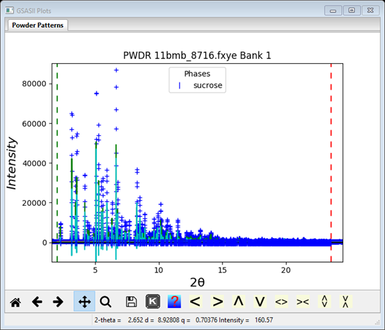
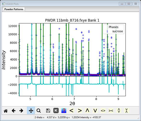
To start the refinement, do Calculate/Refine on the main GSAS-II data tree window. Before it begins a backup of the project file is made; the name will be sucrose.bck0.gpx. It can be used to recover from a bad refinement. A progress dialog box will appear showing the residual as the refinement proceeds. Notice that there was a singular matrix warning on the console window and perhaps the last reflection (781) was removed from the refinement because it was off the end of the used part of the pattern. This is the GSAS-II singular matrix recovery mechanism; you can go to the Pawley reflections tab and uncheck the last reflection. Then repeat Calculate/Refine to make sure it has essentially minimized. My refinement completed with Rwp ~25% (NB: here and after succeeding refinements your Rwp values may be slightly different from what I show here); a dialog box appears asking if you wish to load the result. Press OK. To see the plot select the PWDR line in the GSAS-II data tree (I’ve adjusted the width and height).
It is evident from examining the plot that some improvement can be had by refining the lattice and profile parameters and perhaps the sample X position. Go to Phases/sucrose in the GSAS-II data tree and check the Refine unit cell box. Now select Instrument parameters for the PWDR data set in the GSAS-II data tree and check U, V, W, X & Y. The go to Sample Parameters and check Sample X displ.; make the Goniometer radius 1000 if you didn’t do this earlier. Repeat Calculate/Refine until converged; I obtained an improved residual of ~7.3% with a much better fit at the high angle part of the pattern but still not fit well for the lower part.

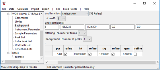
What you see is that the background has a substantial diffuse scattering feature at ~5deg and there are some peak shape issues (which may be a consequence of the poor background fit). We’d like the fit to be better before trying charge flipping. First select Background, set Peaks in background: No. peaks to 1 from the pull down box; the window changes to

Enter 5.0 for pos, 100000 for int and 1000 for sig (as appropriate for broad diffuse peaks) and then check all three refine boxes. Also set No. coeff. pulldown to 5 for the Chebyschev part of the background. The window should look like
Go to the Controls item in the GSAS-II data tree and set the Max cycles to 5. Now do Calculate/Refine until the refinement converges. After a set of refinement cycles go to the Pawley reflections tab and check the intensities. If there are many negatives amongst the highest angle reflections do Pawley update, this replaces all the values with those in the extracted from the profile as listed in the Reflection list for the PWDR data set each multiplied by 0.5. Additionally their refinement flags are turned off. Do Calculate/Refine; this will adjust all the reflections in the vicinity of the reset ones. You may repeat this process to suppress any new negatives that may appear. Then set all the Pawley refinement flags back on (excluding any that lead to a singular matrix) and repeat the refinement. After refinement, mine converged to ~5.3% with very few negatives and the plot looked like

Let’s see if this is good enough for charge flipping.
Step 3: Charge flipping
A few steps are needed to set up for a charge flipping run. Go to Phases/sucrose and notice the Charge flip controls in the middle of the General tab.
1. Select Reflection set from to be PWDR 11bmb_8716.fxye Bank 1 (the only choice!). This makes the reflection set to be used those in Reflection Lists under the PWDR data set; these should match the Pawley reflection set.
2. Set the Peak cutoff (in Fourier map controls) to 20%. This controls the map search routine.
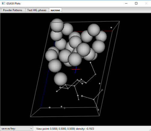
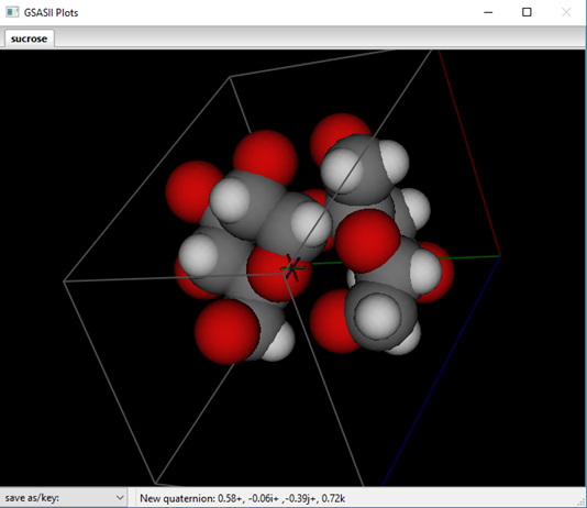
For powder data it is not usually advisable to select a Normalizing element; if selected a periodic table appears – select an element or ‘None’. The Resolution defines the map spacing and thus the extent of the reflection set; the observed reflection set is zero filled to this limit for charge flipping. The k-factor and k-Max determine the lower threshold and upper limit for charge flipping, respectively. The latter is used to avoid “Uranium solutions” in the result. Set this to 10-12 for equal atom problems and larger for heavy atom ones. For sucrose set it to 12. When ready select Compute/Charge flipping; a progress bar dialog will appear that tracks the residual found in each charge flipping cycle. It will quickly drop to some level (42-44%) and then for a successful charge flipping run perhaps drop again into the 20-25% range after a considerable length of time. If it does drop then let it run for a little bit; this “anneals” in the solution and generally gives a better result. You should save the project if you get an apparently good solution. Many times it will not drop below ~40%; just try Compute/Charge flipping again. If several tries fail to yield a solution, go back to the last step of the Pawley refinement and just repeat it (that is do Pawley update and Calculate/Refine). This will generate a different set of intensities for the highly overlapped part of the powder pattern; perhaps they will give a successful charge flip solution. Unless otherwise interrupted, GSAS-II will try 10000 times for a charge flip solution (for sucrose this takes 5-10min on my laptop). Press Cancel to stop the charge flipping; a peak list and a drawing of the solution will appear. One of my runs gave

![]()

The result looks very promising! Charge flipping operates without regard to symmetry and GSAS-II attempts to locate the map with respect to the symmetry elements from the computed reflection phases. (NB: charge flipping also will give a solution without regard to handedness; this solution may be either the correct one for sucrose or its inverse.) Errors in these phases can disrupt this process so that the map and peak positions are offset from their true positions. To discover this and fix it, rotate the drawing around to check that atom positions are related via the 21 screw axis (through the multicolored cross in the center of the cell and parallel to the y-axis – the green cell edge). Avoid motions with the right mouse button pressed, this moves the cross. To recover, press the ‘C’ key to reset the cross to the cell center. I’ve placed the symbol for a 21 axis on my drawing above to show where I think it should be. If you find an offset to the map, orient it so the offset is horizontal or vertical and then press the L, R, U or D keys to shift the map and peaks as needed. The shift is in resolution units (0.5Å) so the fix can only be approximate. Repeat as needed. Notice that the peak positions in the table are updated as the offset is changed. In this case, I needed just a few steps to correct the map offset. NB: you can use these keys to move the result anywhere you wish, e.g. to select a different origin for the structure but pay attention to the location of symmetry elements. After adjustment, my solution looked like

Step 4: Obtain solution from charge flip result
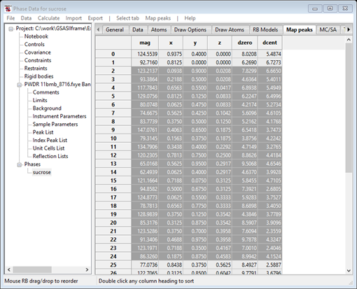
The next step is to extract the unique peak positions from the map and make atoms out of them. The map peak list is initially sorted by peak magnitude; you can change the sorting to be along any of the column headings in the table by a single click on the desired heading. The dzero column gives the distance of each peak from the origin. The menu items under Map peaks give you several tools to aid in the peak selection process; we will just use a couple in this example. I have chosen to proceed by sorting the atoms by z, selecting all and then finding the unique ones.
1. Do a single click on the z column heading. This will sort the peaks in increasing z-axis coordinate.
2. Do a single click on the upper left (empty) box of the table. All entries will be colored grey indicating their selection.
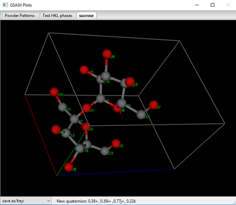
3. Do Map peaks/Unique peaks. That should select (grey) 23 out of 46 peak positions in the table and all should be near the top of the list. The console displays this as both the number of unique peaks and the fraction found (the ideal value, 0.5, for the latter is easily inferred from the space group). Given the formula for sucrose is C12H22O11 that would be all the C & O atoms! They will be colored green in the plot. If more are selected then check the map offset – it may need a slight correction.
The drawing shows the selected atoms in green.

Notice that in my case one atom is in a neighboring molecule, one can deselect it and then pick the desired equivalent. Hold the Shift key down and use the right mouse button to pick/unpick atoms in the drawing. NB: the left mouse button will clear all the selections. The other two “lone” atoms belong to molecules in neighboring unit cells; we’ll deal with them later.
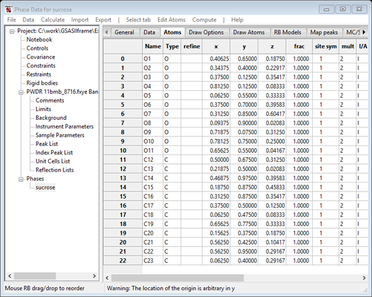
These are now ready to turn into atoms. Do Map peaks/Move peaks. The drawing will show white balls for each of the selected positions and the Atoms table will now have 23 new H atoms.
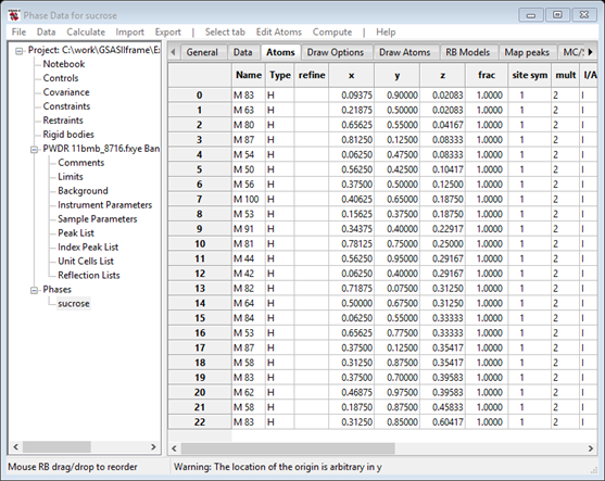
The atom names indicate the peak magnitude to aid identification (M100 for the largest in the Map peaks table which may not be one of those moved to the Atoms table). You can hand sort them by selecting a row with the Alt key (or Shift/Ctrl keys) down and then selecting a position in the table with the Alt key still down. On Linux machines the Alt key may have been hijacked by the operating system; use Shift/Ctrl instead to move atoms. After sorting by magnitude, my list is now

Notice that in this case the atom list is neatly sorted out
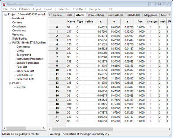
into two groups with a clear gap between M80 and M64. The higher ones are
likely to be the 11 O-atoms and the rest are the 12 C-atoms. There may be a bit
of ambiguity in the middle, but just assign the top 11 as O and the rest as C
and see what happens. You can do this by selecting a block of atoms, go to Edit
Atoms/On selected atoms…/Modify atom parameters and select Type
from the dialog box; a periodic table will appear. Select the desired element
and they will be changed in the list and drawing. 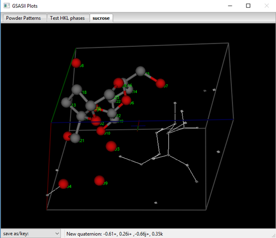
The original charge flipping solution is still visible and the atoms are now identified, I’ve changed the drawing to show balls and sticks and labeled the atoms with their names, this is done in the Draw atoms tab. Double click the appropriate column heading and make the selection from the dialog box.
Now one can safely remove the map peaks (do Map peaks/Clear peaks in the Map peaks tab) and clear the charge flip map (do Clear map in the General tab). The atom positions I obtained in this charge flipping run have the sucrose molecule fragmented over several neighboring molecules. We need assemble these into a single molecule. Follow the steps:
1. In the Atoms tab of the Data window do Edit Atoms/Reload draw atoms. This ensures the drawing is up-to-date with the Atom list.
2. Select one atom in one of the fragments (perhaps O(1) in the drawing above as that is likely to be the bridging O-atom between the two rings of sucrose. With the Atoms table showing on the data window, use Shift-Left mouse button on the desired atom; it will turn green indicating selection.
3. Then in the Atoms menu do Edit Atoms/Assemble molecule; a popup dialog offering choices of distances (& angles – not used). Press Ok.
The atoms will automatically be reorganized into a single molecule and are ordered in the table according to connectivity.
I’ve changed the style to balls & sticks and added the atom names as labels.
If it happens that the Assemble molecule routine leaves one or two atoms out, rerun it adjusting the Bond search factor to a slightly larger value (e.g. 0.9 vs 0.85). That should pick up the outliers.
To rename the atoms, select all the atoms (double click in the empty left upper square of the Atom table; the entries will turn blue or grey. Then do Edit Atoms/On selected atoms…/Modify atom parameters. Select Name from the popup window and press OK; you will be asked to confirm. The atoms will be renamed.

You can also reorder the atoms to make the connectivity conform to usual chemical naming rules; use the Alt key to pick & place each atom to be moved just as we did with the Map peak results above.
Save the project file; the next step is to complete the structure by finding H-atoms and then do the final Rietveld refinements.
Step 5: Complete the structure
To complete the structure you will need to perform a preliminary Rietveld refinement. This will make the atom positions more accurate and prepare a set of calculated structure factors needed to generate a difference Fourier map good enough to maybe reveal the H atoms. There are a number of steps needed to set all the controls from the previous Pawley refinement to get a successful start for the Rietveld refinement.
1. Go to the Instrument Parameters entry in the GSAS-II data tree and uncheck all Refine boxes. You don’t want to start with these when the scale factor is unknown.
2. Go to Sample Parameters and check the Histogram scale factor box. This is the scale factor for the data set. Uncheck the Sample X displ.
3. Go to Phases/sucrose General tab and uncheck Refine unit cell and Do Pawley refinement boxes. The latter is most important; if you forget you will just get another Pawley refinement!
Now do Calculate/Refine from the main GSAS-II data tree menu; only scale and background are refined. I got Rwp ~25%. The plot shows clear intensity differences; the atom positions obviously need refinement.
I’ve shifted & zoomed in to make the differences more obvious.
Go to Phases/sucrose and select the Atoms tab. Note the warning at the bottom of the window; the origin in space group P21 has an arbitrary location along the y-axis. Then double click the refine column heading, a dialog box will appear, select the X-coordinates box and press OK. The atoms table will show the refinement controls

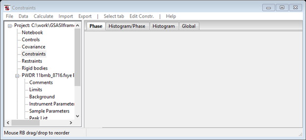
To deal with the warning we need to set a “Hold” on one atom y-coordinate. Select Constraints in the main GSAS-II data tree; the Phase tab is the one we want here.
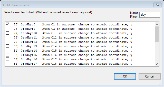
Do an Edit Constr./Add hold and select ‘0::dAy:0 for O(1)’ from the dialog box. Notice the use of a filter to shorten the list. This will fix the shift along y for the O(1) atom.
Press OK; the Constraints window will show the hold

Do Calculate/Refine again; my Rwp is now ~10.3%. You can now safely refine lattice parameters (in the General tab for Phases/sucrose), the Instrument parameters U, V, W, X & Y and the Sample X displ. You can also include refinement of atom thermal motion (Uiso) parameters. My refinement improved slightly to Rwp~10.0%. Next we should add the hydrogen atoms that are on carbon as these can be located from the molecular geometry. To do this do the following:
Go to the Atoms tab and select the Type column; a popup will appear. Select just the C atoms; these will be highlighted in grey in the Atom table.
Do Edit Atoms/On selected atoms…/Calc H atoms from the menu; a Distance Angle
Controls popup will appear. You can change radii and Bond search factor if
needed (rarely). Press Ok. A new popup window will
appear.

This offers the choice of how many H-atoms to be added for each atom in the
table; the maximum is chosen for each atom. If the bonds are sufficiently short
this may be fewer reflecting the possibility of sp2 or sp bonding on the atom. You can override the choices made
by default. You also can deselect some of the other attached atoms so they will
not be used in the geometry calculations for H-atom placement (e.g. a metal
atom in certain organometallics). When you are satisfied with the choices
(actually no changes are needed in this case), press Ok. The structure will
be redrawn with H-atoms shown as van der Waals spheres; they are inserted in
the Atom list immediately after the C-atom they are bound to and they are named
accordingly.
These hydrogen atoms will better describe the scattering density in the vicinity of the carbon atoms; their positions need to be refined to find their better locations. Do Calculate/Refine (the refinement flags are already set for this – NB: don’t be tempted to refine the H-atom positions as they are likely to move erratically). My result was Rwp~9.2% and the drawing is updated with the new atom positions (as van der Waals spheres).

Because the C-atoms have probably moved; the H-atoms (which were fixed) are now no longer in their optimal locations. From the menu, do Edit Atoms/ pdate H atoms. This will shift their positions slightly. Repeat Calculate/Refine and Edit/Update H atoms; you should see no shift this time. (Rwp may be slightly higher; I got ~9.3%).
Now we have to find the hydrogens that are on oxygen; these cannot be geometrically located except that they are somewhere on a circle at the bonding distance from the O-atom. We need a difference Fourier map. Go to the Phases/sucrose General tab; the Fourier map controls are midway down the window.
1. Select delt-F for the Map type.
2. Select PWDR 11bmb_8716.fxye Bank 1 for the Reflection set from item (the only choice). The Fourier calculation will use the structure factors shown in the Reflection list item for this PWDR data set.
3. Do Compute/Fourier map from the General tab window. The map will be computed via fast Fourier techniques and is very fast. A few lines summarizing the map is printed on the console, the structure plot may show a single green dot somewhere (it could be hidden beneath an atom!), this is the highest point in the map.
4. Go to the Draw Options tab and adjust the Contour level slider until something appears on the map. You can also reduce the Map radius and shift the View Point (use right mouse button) to help clarify the view. Note that the map continues to show the density around the View Point even if it is outside the unit cell box.

What is drawn here are green (& red for negative) dots whose size are proportional to the electron density. There are peaks that might be H-atom positions as well as features that suggest O-atoms out of position. Recall that the refinement was just done without any H-atoms on the oxygen atoms; it will make the best fit compensating for the missing H-atoms by displacing the O atoms in the direction of the missing H-atoms. To add the OH atoms do the following:
1. Go to the Phases/sucrose Atoms tab.
2. Select all O-atoms in the table (double click the Type column heading & select O atoms from the popup); all will turn grey.
3. Do Edit Atoms/On selected atoms…/Calc H atoms from the menu; a Distance Angle Controls popup will appear. You can change radii and Bond search factor if needed (rarely). Press Ok. A new popup window will appear
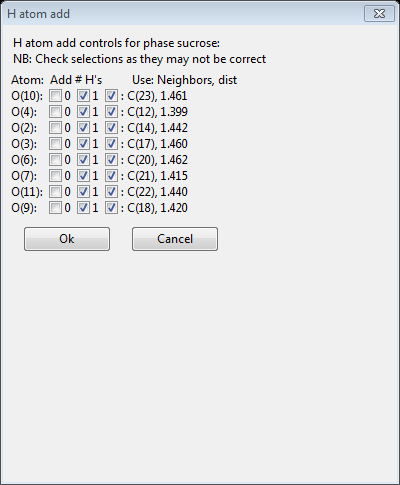
This offers the choice of how many H-atoms to be added for each O-atom in the table; one is chosen in this case for each atom. Press Ok. The structure will be redrawn showing the added H-atoms.
These OH hydrogens are found by finding the highest point in the delta-F map for all possible orientations of this bond at a fixed angle (109.5°). The new hydrogen atoms are inserted in the Atom list immediately after the O-atom they are bound to and they are named accordingly
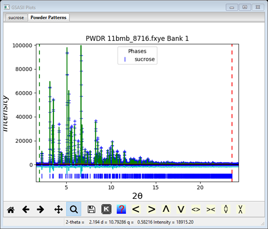
Do the set of Calculate/Refine, Edit Atoms/Update H atoms at least twice to finish this stage in the structure analysis; end with a Calculate/Refine. My Rwp was ~8.14% with all the H-atoms included (but not refined). The fit looks pretty good
Step 6: Final refinement
Looking at the fit, there may be room for improvement. First we need to change the profile model to include crystallite size and mustrain broadening. Go to Instrument Parameters, set X and Y to zero and uncheck the Refine flags for them.
Next go to Phases/sucrose and look at the Data tab. Check the boxes for both Cryst. size and microstrain.
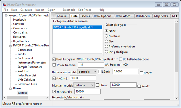
Do a Calculate/Refine; the Rwp will start out high but should converge to where it was before this change. I got 8.09% and the Data tab looked like

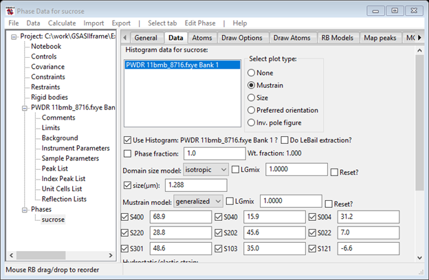
Next select Generalized for the Mustrain model; this is the Stephens phenomenological model for microstrain which has 9 terms for monoclinic structures. Check all the boxes for it and press Reset. This will convert the isotropic strain value to the equivalent generalized values.
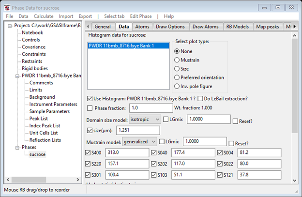
Do a Calculate/Refine; the Rwp will start out high but should converge lower than where it was before this change. I got 7.65% and the Data tab looked like. If you check the Mustrain button in the Select plot type box, you will see the interesting mustrain surface plot for ground sucrose.

This completes the exercise.